The kidneys are vital organs responsible for excretion, fluid and electrolyte balance and hormone production. The nephrons are the kidney's functional and structural units. The number, size and distribution of the nephron components contain relevant information on renal function. Stereology is a branch of morphometry that applies mathematical principles to obtain three-dimensional information from serial, parallel and equidistant two-dimensional microscopic sections. Because of the complexity of stereological studies and the lack of scientific literature on the subject, the aim of this paper is to clearly explain, through animal models, the basic concepts of stereology and how to calculate the main kidney stereological parameters that can be applied in future experimental studies.
Los riñones son órganos vitales que realizan funciones de excreción, equilibrio hidroelectrolítico y producción de hormonas. La nefrona es su unidad estructural y funcional. El número, tamaño y distribución de los componentes de la nefrona contienen información relevante sobre la función renal. La estereología es una rama de la morfometría que permite, aplicando reglas matemáticas, obtener información tridimensional de estructuras biológicas a partir de cortes microscópicos bidimensionales, seriados, paralelos y equidistantes. Ante la complejidad de los estudios estereológicos y la carencia de una bibliografía clara sobre el desarrollo de los mismos, el objetivo de este trabajo es explicar de forma sencilla y con ejemplos, utilizando un modelo animal, los conceptos básicos de estereología, así como el cálculo de los principales parámetros estereológicos renales y que estos puedan ser aplicados en futuros estudios experimentales.
Kidneys are an essential organ in the maintenance of homeostasis, and nephrons are their structural and functional unit. The number, size, and distribution of nephron components (glomeruli, tubules, …) provide important information about renal function, making their quantification important in studies of traumas, chemicals and/or diseases. In these cases, as well as under normal circumstances, stereological studies allow us to detect and quantify macro- or microscopic changes.1
Stereology is a part of morphometry that allows three-dimensional information of cells or other biological structures to be collected from two-dimensional, serial, parallel, and equidistant microscopic slices by applying mathematical formulas based on statistically significant geometrical probability.2
Given the difficulty of stereological studies and the lack of a clear bibliography on their development, the objective of this work is to explain how to calculate the main stereological parameters of the kidney, step by step, in a simple manner and with examples utilising an animal model; the idea is to establish easily understandable bases applicable in experimental studies. This will contribute to the resolution of many pathological, physiological, and biochemical problems.2,3
Material and methodsSample preparationRat kidneys are extracted and fixed for 24h in 4% paraformaldehyde at room temperature. They are subsequently washed with water. Will undergo successive ethyl alcohol baths with increasing concentrations; then they are cleared with xylol and embedded in paraffin (each kidney in a separate mould). Once the blocks are made, they are kept in cabinets at room temperature.
Preparation of histological slicesIt is best to start with a pilot study that includes one or two animals, to gradually correct errors and adjust the steps (for example, how many fields we will use to measure glomeruli, how many dissectors per histological field, etc.).4
We place a block with a kidney in the microtome and cut all of it into 5-μm thick sections. Orientation does not influence the calculation of the volume and numerical density1 (in our laboratory we make cross sections). Another problem that may arise when tackling this objective is whether or not it is necessary for the renal cortex to be isotropic in order to apply the method and whether the size of the particles may lead to an error.
As has been explained previously in classic articles,5 that problem can be solved with adequate sampling, which gives each particle, in this case glomeruli, the same probability of being counted.
For the stereological study, we will divide the sections or slices number 100 and 106, 200 and 206, … and successively in the same manner until the end.
We will choose only those slices that are not broken or folded when laying them out on the slide. If this happens with the slice that we are supposed to select, we will advance 5μm or whatever is necessary to obtain an optimal slice, as long as we then maintain the distance of 25μm with its corresponding paired section, and we continue with the initially established system.
The sections 100, 200, … are to calculate the total volume of the kidney or the Cavalieri reference volume, and we will call them “volume sections”. They are obtained systematically (there is always the same distance between the slices or T), uniformly (each of the slices are parallel) and randomly (the first slice is chosen arbitrarily between the slices 0 and T, with T being the same as 100 slices in this case). It is important to obtain a minimal number of slices (greater than or equal to 6) needed to obtain a volume with an acceptable error coefficient.1,3,4
Sections 106, 206, … are paired sections that will be used to estimate the numerical density (number of glomeruli/mm3) according to the physical dissector method. The reason why they are separated 6 slices from their pair section (“volume section”) is because the optimal distance between these sections must be approximately 1/3 of the mean diameter of the structure to be measured (in this case, the glomerulus).6 In the case of kidney glomeruli in adult rats, this would be about 25μm7,8 (at 5 slices with a thickness of 5μm). The 2 paired sections are placed on the same slide.
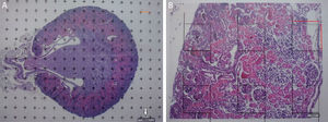
Stereological analysisTo calculate the total volume we will make photomicrographs of the “volume sections” where the entire kidney can be seen (1× and 1.25× objective). Each photograph must incorporate its corresponding scale. We will superpose a point grid over them with which we will calculate the distance between each point or mark and will call it Δx, and measure the distance in mm with a gauge (Fig. 1A). Once we have the grid over the kidney, we count the number of points or marks that “fall” over the image of the kidney (we will call it ∑P).
(A) Photomicrograph with a 1.25× objective of a cross-section of a mouse kidney (haematoxylin–eosin), with a superposed point grid for counting the points and calculating the Cavalieri volume. White arrow: scale present for calculating the magnification. Red line: Δx or distance between points. (B) Photomicrograph of a histological field with 10× objective of the renal cortex according to the cross section, with superposed grid with 6 dissectors. Red line: Δx and Δy (the same since they are a square dissector).
Since the photomicrograph may be larger or smaller depending on the size of the monitor where it is projected, we use the scale of the photograph to keep it from affecting the study, and we measure it on the monitor with a gauge. With that measurement we can calculate the magnification or M:
Now, we are ready to apply the following formula:
T=distance between “volume sections”.
a/p (area associated with each point), Δx2 is the distance between two points of the grid and M is the magnification.
∑P=sum of points falling within the structure to be measured (kidney), superposing a point grid on it, in each of the resulting photographs (for example, if we have 6 “volume sections”, then ∑P=∑P1+⋯+∑P6).
In order to calculate the numerical density according to the physical dissector method,1,6,7 we apply a grid with the dissectors over the photomicrographs of slices 100, 200, … (“reference sections”) and then we compare them with their pairs 106, 206, … (“look up” sections). To do this, we make 2 photomicrographs (10× objective) of each paired section (always with the scale) that will allow us to simultaneously see the 2 sections. Once we have located the same histological area in both paired slices, we superpose the template with the 6 dissectors (could be more or less) on the reference image (100, 200, …) and count how many glomeruli (∑Q−) of the reference image (Fig. 1A) fall within the counting frame without touching the forbidden lines (straight lines) and do not appear in the “look up” image (Fig. 1B).
This should be done on 10 random cortical fields of each “volume section” obtained (looking for histological references to ensure the same location in the 2 paired sections).
For the study to be well done, we have to count between 100 and 200 glomeruli or ∑Q−, because thus, when the formula for calculating the error coefficient or estimating the variance error is applied, it would have an approximate value of 0.1.
Finally, we count the number of dissectors (∑P) used in the glomerular count to calculate on which kidney volume the glomeruli are being counted. In the example case they would be: 60 dissectors for each “volume section” (6 dissectors superposed on 10 histological fields)×total number of “volume sections” that we have obtained.
Finally, we apply the following formula to obtain the numerical density:
a/f(count or dissector framework area)=Δx×ΔyM2.
h: distance between paired sections of the dissector (in this case, 25μm).
∑Q−: sum of particles or glomeruli counted according to the dissector, in every “volume section”.
∑P: sum of dissectors used to measure the glomeruli in every “volume section”.
Once we have the numerical density (Nv), we can make an estimate of the total number of glomeruli3,4:
ResultsWe began by sectioning the kidney of an 0F1 adult mouse (Charles River, Barcelona, Spain) in 5-μm thick sections, with a T of 500μm (equivalent to 100 separation slices between “volume sections”).
Total volume calculation according to CavalieriDue to the size of the kidney, we obtained 10 “volume sections” and photographed them with a 1.25× objective on the microscope, incorporating the scale (which for this objective corresponds to a scale of 500μm, and measured on the photo are 15.5mm).
We applied the point grid and made the following count (Table 1).
Values of the points on the cortex and renal medulla for calculating the total volume of the example. And number of glomeruli and dissectors used to calculate the numerical density of the example.
| Histological slice | Points over cortical | Points over medullar | Histological slice | Number of glomeruli | Number of dissectors |
|---|---|---|---|---|---|
| 1 | 46 | 0 | 1 | 19 | 24 |
| 2 | 107 | 51 | 2 | 17 | 40 |
| 3 | 101 | 86 | 3 | 23 | 39 |
| 4 | 116 | 97 | 4 | 19 | 40 |
| 5 | 111 | 77 | 5 | 20 | 39 |
| 6 | 94 | 86 | 6 | 22 | 32 |
| 7 | 105 | 58 | 7 | 26 | 40 |
| 8 | 96 | 77 | 8 | 29 | 40 |
| 9 | 94 | 57 | 9 | – | – |
| 10 | 65 | 0 | 10 | – | – |
| Total (∑P) | 935 | 589 | Total | 175 | 294 |
| Cortical+medullar | 1524 | ||||
With this data we are able to calculate:
T=500μm or 0.5mm.Calculation of the numerical density with the physical dissectorWe took 2 photomicrographs (10× objective) of each paired section (scale of 200μm that measured 41mm). We located the same histological area in both paired slices, superposed the template with the 6 dissectors on the “reference image” (100, 200, …) and counted how many glomeruli (∑Q−) fall within the counting frame without touching the forbidden lines (straight lines) and do not appear in the look up image (paired section). We repeated this action over 10 fields of each “volume or reference section”.
We counted the number of dissectors utilised and applied the formula:
Conflicts of interestThe authors declare that they have no conflicts of interest.
The authors would like to the thank the collaboration of Dr. Jorge Arias and Dr. Marta Méndez, of the Psychology Department of the Universidad de Oviedo [Oviedo University], and especially Professor Luis M. Cruz-Orive, of the Universidad de Santander [Santander University].
Please cite this article as: Fernández García MT, Núñez Martínez P, García de la Fuente V, Sánchez Pitiot M, Muñiz Salgueiro MdC, Perillán Méndez C, et al. Aplicación práctica de métodos estereológicos renales en modelos animales experimentales. Nefrologia. 2017;37:29–33.


